Poisson CPP

C++20 library of Poisson solvers : finite volume, spectral, AMR + multigrid, Conjugate Gradient.

_{Scène multi-charges (10 gaussiennes ±q) résolue par le solveur AMR : 5 287 feuilles quadtree, SOR convergé à 10⁻⁸ en 300 itérations. Fond = |V| (viridis), courbes = équipotentielles, points rouges = charges. Reproduction : python/make_banner.py.}

Solveurs

Module	Algorithme	Coût	BC supportées
`linalg::thomas`	Tridiagonal direct	O(N)	toutes
`fv::Solver1D`	FV + Thomas	O(N)	Dirichlet (ε uniforme ou variable)
`fv::Solver2D`	FV + SOR red-black ω_opt	O(N³)	Dirichlet×Neumann
`iter::solve_poisson_cg`	CG / PCG Jacobi	O(N³), ~5× SOR	Dirichlet×Neumann
`spectral::DSTSolver2D`	DST-I via FFTW	O(N²·logN)	Dirichlet homogène
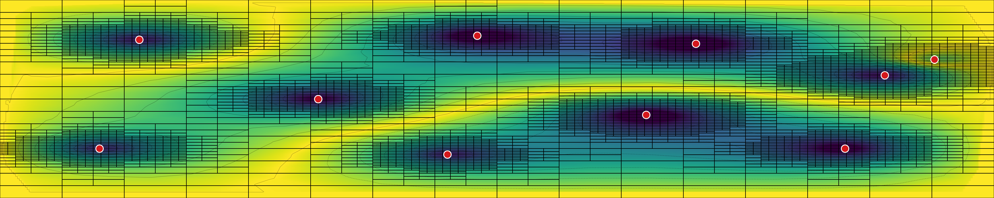
`amr::Quadtree` + `sor`	Quadtree Morton + FV hétérogène	O(nb_leaves × iter)	Dirichlet V = 0 au bord
`mg::vcycle_amr_composite`	V-cycle 2-grid composite AMR	O(nb_leaves) par cycle	Dirichlet V = 0

Tous matrix-free. Pseudocode de chaque solveur : **docs/ALGORITHMS.md**. Conventions de grille et schémas modules : docs/ARCHITECTURE.md.

Documentation

Python (Sphinx) : https://wolf75222.github.io/poisson_cpp/
C++ (Doxygen) : https://wolf75222.github.io/poisson_cpp/cpp/

Quick start

Prérequis

C++20 (AppleClang 16+, GCC 12+, Clang 15+, MSVC 19.36+)
CMake ≥ 3.20
Eigen ≥ 3.4 *(fetched automatiquement si absent)*
FFTW3 *(optionnel, active le solveur spectral)*
OpenMP *(optionnel, parallel sweeps à partir de N ≥ 384)*
Python 3.9+ *(optionnel, bindings pybind11)*

Build

git clone https://github.com/wolf75222/poisson_cpp.git
cd poisson_cpp
cmake -B build -DCMAKE_BUILD_TYPE=Release
cmake --build build -j
ctest --test-dir build                              # 66 tests C++ doivent passer
pytest tests/python                                  # 50 tests Python (après pip install .)

Options CMake :

Option	Défaut	Rôle
`POISSON_BUILD_TESTS`	`ON`	Compile Catch2 + toute la suite
`POISSON_BUILD_BENCHMARKS`	`ON`	Compile `bench_solvers` et `profile_cg`
`POISSON_USE_OPENMP`	`OFF`	Parallélise SOR + gs_smooth au-delà de N ≥ 384
`POISSON_BUILD_PYTHON`	`OFF`	Génère le module `poisson_cpp` via pybind11

Exécuter le démo C++

# 1D Poisson + dump JSON
./build/examples/poisson_demo --problem poisson1d --N 100 --uL 10 --uR 0 \
    --output /tmp/p1d.json
 
# SOR 2D avec historique de convergence
./build/examples/poisson_demo --problem sor2d --N 128 --uR 10 --tol 1e-10
 
# Spectral 2D (nécessite FFTW)
./build/examples/poisson_demo --problem spectral2d --N 256
 
# Scène AMR multi-charges (utilisée pour la bannière)
./build/examples/poisson_demo --problem amr_scatter --Nmin 4 --Nmax 7 \
    --sigma 0.025 --output data/snapshots/amr_scatter.json

Utilisation depuis Python (pybind11)

Installation pip

pip install git+https://github.com/wolf75222/poisson_cpp.git

Le wheel est compilé localement par scikit-build-core. Prérequis : compilateur C++20 et CMake ≥ 3.20. Eigen et nlohmann_json sont récupérés automatiquement. FFTW3 est optionnel ; sans lui, DSTSolver1D/2D sont désactivés et un RuntimeWarning à l'import donne la commande d'installation pour ta plateforme.

Google Colab

!apt-get install -y libfftw3-dev > /dev/null     # optionnel, pour le DST
!pip install git+https://github.com/wolf75222/poisson_cpp.git
 
import numpy as np, poisson_cpp as pc
g = pc.Grid2D(1.0, 1.0, 64, 64)
V, rep = pc.Solver2D(g, eps=1.0, uL=0.0, uR=10.0).solve(np.zeros((64,64)), tol=1e-8)
print(rep)

Si FFTW est installé après coup, force la recompilation :

pip install --force-reinstall --no-binary poisson-cpp poisson-cpp

Build manuel depuis les sources

cmake -B build -DPOISSON_BUILD_PYTHON=ON
cmake --build build --target poisson_py -j
export PYTHONPATH=$PWD/build/python

Exemple

import numpy as np
import poisson_cpp as pc
 
# ---- 1. Thomas (tridiagonal direct, 1D) --------------------------------
N = 100
a = np.zeros(N); b = 2.0 * np.ones(N); c = np.zeros(N); d = np.ones(N)
a[1:] = -1.0; c[:-1] = -1.0
x = pc.thomas(a, b, c, d)
print("thomas:", x[:3])                    # [1.0, 2.0, ... ]
 
# ---- 2. Solver2D : FV + SOR red-black ω_opt auto -----------------------
grid = pc.Grid2D(1.0, 1.0, 64, 64)         # [0,1]² cell-centered
sor  = pc.Solver2D(grid, eps=1.0, uL=0.0, uR=10.0)   # Dirichlet x, Neumann y
rho  = np.zeros((64, 64))
V, report = sor.solve(rho, tol=1e-10)      # returns (V, SORReport)
print(report)                              # SORReport(iterations=..., residual=...)
 
# ---- 3. Conjugate Gradient --------------------------------------------
V_cg = np.zeros((128, 128), order="F")     # Fortran-order pour Eigen in-place
grid = pc.Grid2D(1.0, 1.0, 128, 128)
rep, hist = pc.solve_poisson_cg(
    V_cg, np.zeros((128, 128), order="F"), grid,
    uL=0.0, uR=10.0, tol=1e-10, record_history=True)
print(f"CG: {rep.iterations} iterations, residual {rep.residual:.2e}")
 
# ---- 4. Spectral DST-I (si FFTW disponible) ----------------------------
if pc.has_fftw3:
    dst = pc.DSTSolver2D(127, 127, 1.0, 1.0, eps0=1.0)
    rho_dst = np.random.randn(127, 127)
    V_dst = dst.solve(rho_dst)
    print("DST2D V range:", V_dst.min(), V_dst.max())

Plots

python3 python/plot_figures.py all            # toutes les figures de validation
python3 python/plot_cg.py                     # convergence CG vs SOR
python3 python/make_banner.py                 # bannière AMR multi-charges

Figures dans docs/figures/, interprétations dans `docs/RESULTS.md`.

Résultats



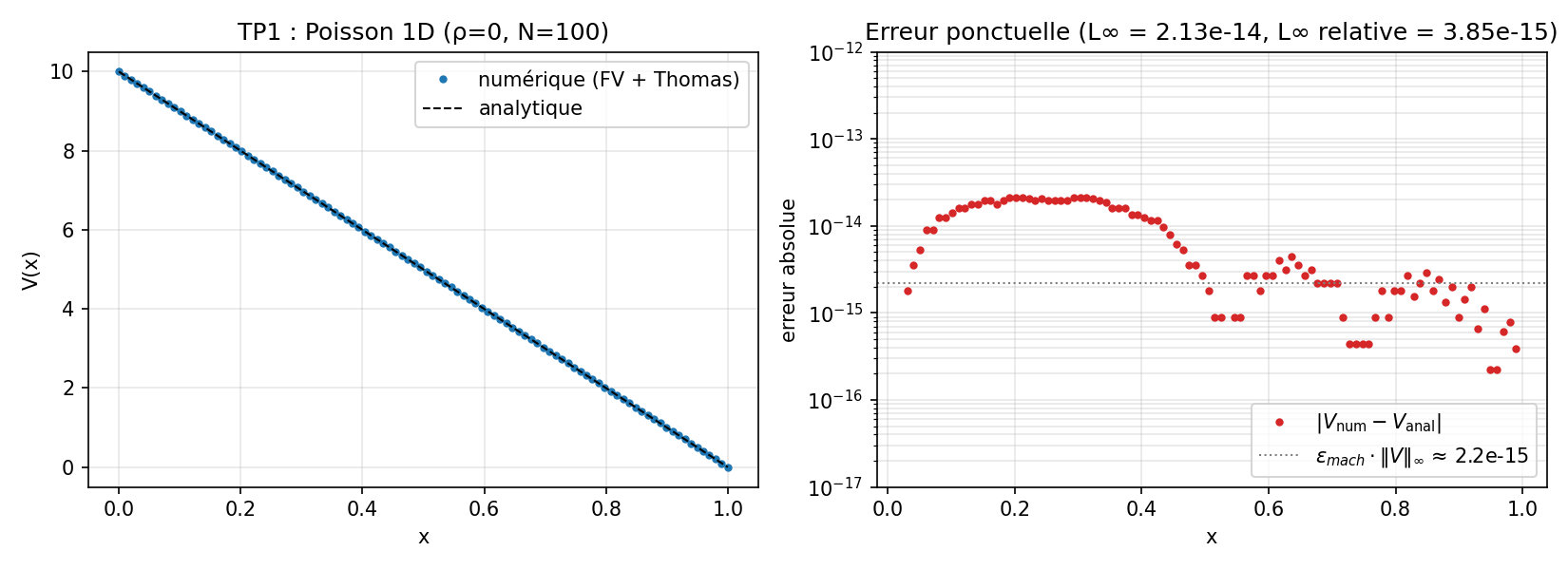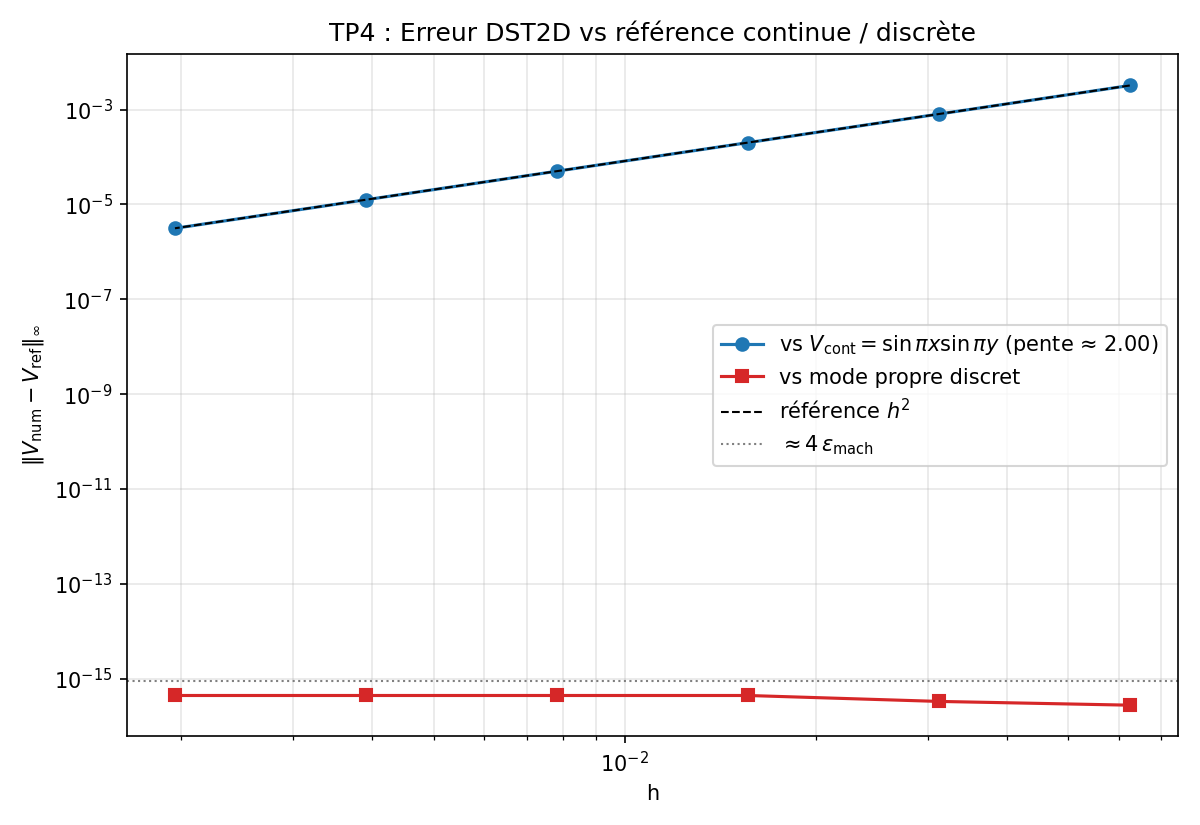Poisson 1D, erreur L∞ = 2.1×10⁻¹⁴ (précision machine)	Convergence spectrale, pente log-log = +2.000

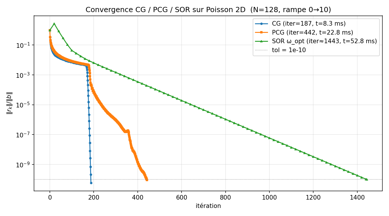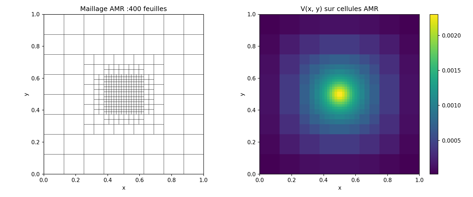CG : 187 iter / 8 ms vs SOR 1443 / 53 ms	AMR sur Gaussienne centrée, 400 feuilles, ×10 vs uniform

Performance

Détails dans `docs/PERFORMANCE.md`. A/B mesurés avec sample / xctrace :

mg::gs_smooth N=128 : in-place red-black, −68 %.
Solver2D::solve N=128 : in-place red-black + Vc_inv_ précomputé, −46 %.
amr::sor : précalcul rhs = h²ρ/ε₀ et Vc_inv, −16 %.
Solver2D::solve : fold Dirichlet → rhs pour débloquer SIMD, −5 %.
CG apply_neg_laplacian N=512 : diag_mat précomputé hors hot loop, −18 %.
OpenMP (opt-in, N ≥ 384) : Solver2D + gs_smooth, ×1.5 à ×1.9.

Tests

66 tests Catch2 côté C++ + 50 tests pytest côté bindings Python. Couvrent :

Invariants mathématiques (réciprocité de Green, linéarité, symétrie de réflexion) à 1e-13.
Lois de conservation (Gauss, énergie, continuité D aux interfaces diélectriques) à 1e-12.
4 snapshots JSON vs les notebooks Python à 1e-10.
Convergence O(h²) sur un benchmark Fourier (Jackson ch.2).
Scaling CG en O(N), cross-check vs DST.
Côté Python : workflow AMR + multigrille bout-en-bout, dataclasses, helpers (Morton, harmonic_mean, dump_amr_snapshot).

ctest --test-dir build # C++

pytest tests/python # Python

Détails : `docs/RESULTS.md` (figures de validation), `docs/PERFORMANCE.md` (benchmarks A/B + profiling).

License

BSD-3-Clause. Voir [LICENSE](LICENSE).